Geo Numeracy
Working with geometry using numpy, and other musings.
Maintained by Dan-Patterson
Clipping
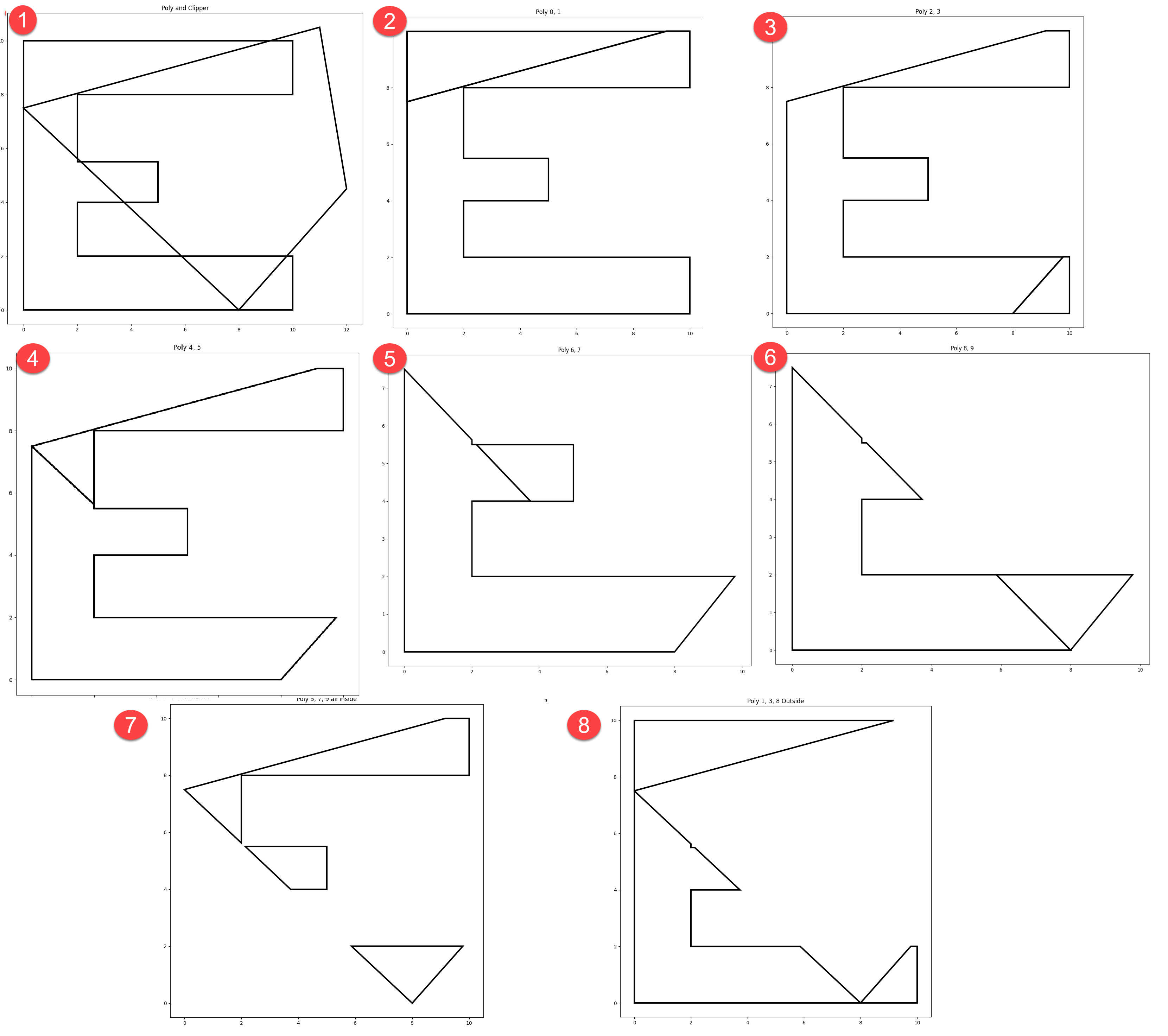
The image to the right shows the results of intersecting two sets of segments which coincedently form two polygons.
The sequential steps show how each segment of the clipper intersects with the segments of poly.
The clips are keep in a left of and right of containers (read... outside vs inside).
The right of data are used in the next clipping step... and so on, and so on.
At the end, it is simply a matter of organizing the outside and inside bits (aka, erase and clip).
Note the word simply. This is where the yeah but... comments start.
All the corner cases, where things aren't so simple.
The journey begins.
The intersection points between the point sets was determined using p_c_p below.
The coordinates for the inputs are.
#      poly                  clipper
array([[  0.00,   0.00],   array([[  0.00,   7.50],
       [  0.00,  10.00],          [ 11.00,  10.50],
       [ 10.00,  10.00],          [ 12.00,   4.50],
       [ 10.00,   8.00],          [  8.00,   0.00],
       [  2.00,   8.00],          [  0.00,   7.50]])
       [  2.00,   5.50],
       [  5.00,   5.50],
       [  5.00,   4.00],
       [  2.00,   4.00],
       [  2.00,   2.00],
       [ 10.00,   2.00],
       [ 10.00,   0.00],
       [  0.00,   0.00]])
They can be rearranged to form the raveled point pairs, which are useful for some functions
np.concatenate([poly[:-1], poly[1:]], axis=1)
np.concatenate([clipper[:-1], clipper[1:]], axis=1)

#  poly as segments                           clipper as segments
array([[  0.00,   0.00,   0.00,  10.00],  array([[  0.00,   7.50,  11.00,  10.50],
       [  0.00,  10.00,  10.00,  10.00],         [ 11.00,  10.50,  12.00,   4.50],
       [ 10.00,  10.00,  10.00,   8.00],         [ 12.00,   4.50,   8.00,   0.00],
       [ 10.00,   8.00,   2.00,   8.00],         [  8.00,   0.00,   0.00,   7.50]])
       [  2.00,   8.00,   2.00,   5.50],
       [  2.00,   5.50,   5.00,   5.50],
       [  5.00,   5.50,   5.00,   4.00],
       [  5.00,   4.00,   2.00,   4.00],
       [  2.00,   4.00,   2.00,   2.00],
       [  2.00,   2.00,  10.00,   2.00],
       [ 10.00,   2.00,  10.00,   0.00],
       [ 10.00,   0.00,   0.00,   0.00]])
Or they can be shaped to from 3D arrays of coordinates of from-to pairs.
np.concatenate([poly[:-1], poly[1:]], axis=1).reshape(-1, 2, 2)
np.concatenate([clipper[:-1], clipper[1:]], axis=1).reshape(-1, 2, 2)

#  poly as from-to point pairs    clipper as from-to point pairs
array([[[  0.00,   0.00],         array([[[  0.00,   7.50],
        [  0.00,  10.00]],                [ 11.00,  10.50]],
       [[  0.00,  10.00],                [[ 11.00,  10.50],
        [ 10.00,  10.00]],                [ 12.00,   4.50]],
...    snip                       ...    snip
       [[ 10.00,   2.00],                [[  8.00,   0.00],
        [ 10.00,   0.00]],                [  0.00,   7.50]]])
       [[ 10.00,   0.00],
        [  0.00,   0.00]]])
The resultant intersections between the segments are shown below.
If you examine the poly ID and clip ID columns and the figure above, you will see how one can sequentially construct
a clip or erase from the intersection points and the point inside and/or outside their respective segments.
Steps 7 and 8 in the image represent the cases where segments that are inside the clipper bounds are kept
(clip, step 7) or are removed (erase, step 8).
How you can assemble the bits for form polygons will be the subject of a subsequent document.
I won't become obvious anytime soon, but study the coordinates, their arrangements, the intersections and the image in the interim.
The order of the ID values in the listing below is organized by the poly ID values.
This shows the first poly segment (0) was intersected by the first and third clipper (0, 3).
The second poly segment (1) was intersected by the first clipper (0). Poly segments 2 and 3
had no intersection points ... and so on.
Understand the structure of how the IDs can be arranged.. by poly or by clipper... since they are both useful.
More later.
# intersections            poly clip
#          X       Y        ID   ID
array([[  0.00,   7.50],   [ 0,   0],
       [  0.00,   7.50],   [ 0,   3],
       [  9.17,  10.00],   [ 1,   0],
       [  2.00,   5.62],   [ 4,   3],
       [  2.13,   5.50],   [ 5,   3],
       [  3.73,   4.00],   [ 7,   3],
       [  9.78,   2.00],   [ 9,   2],
       [  5.87,   2.00],   [ 9,   3],
       [  8.00,   0.00],   [11,   2],
       [  8.00,   0.00]]), [11,   3]
The basic code to perform the intersections is listed in p_c_p (poly-clips-poly).
The seemingly strange notation dc[:, 0][:, None] is used to produce a broadcastable data structure
that enables one to perform operations of arrays of varying shapes. [1]
def p_c_p(clipper, poly):
    """intersect poly features.

    Parameters
    ----------
    clipper, poly : array_like
         Clockwise-ordered sequence of points (x, y) with the first and last
         point being the same. The `clipper` is the polygon or polylines
         cutting the `poly` geometry.
    """
    p_cl, c_cl = [i.XY if hasattr(i, "IFT") else i for i in [poly, clipper]]
    x3_x2, y3_y2 = (p_cl[1:] - p_cl[:-1]).T
    dc = c_cl[1:] - c_cl[:-1]
    dc_x = dc[:, 0][:, None]
    dc_y = dc[:, 1][:, None]
    pc02 = p_cl[:-1] - c_cl[:-1][:, None]
    pc02_x = pc02[..., 0]
    pc02_y = pc02[..., 1]
    # --
    d_nom = (x3_x2 * dc_y) - (y3_y2 * dc_x)
    a_0 = pc02_y * dc_x
    a_1 = pc02_x * dc_y
    b_0 = x3_x2 * pc02_y
    b_1 = y3_y2 * pc02_x
    a_num = a_0 - a_1  # (p02_y * dc_x) - (p02_x * dc_y)
    b_num = b_0 - b_1  # (x3_x2 * p02_y) - (y3_y2 * p02_x)
    with np.errstate(all='ignore'):  # divide='ignore', invalid='ignore'):
        u_a = a_num/d_nom
        u_b = b_num/d_nom
        z0 = np.logical_and(u_a >= 0., u_a <= 1.)
        z1 = np.logical_and(u_b >= 0., u_b <= 1.)
        both = z0 & z1
        xs = u_a * x3_x2 + p_cl[:-1][:, 0]
        ys = u_a * y3_y2 + p_cl[:-1][:, 1]
    xs = xs[both]
    ys = ys[both]
    pc_ids = np.vstack(both.nonzero()).T
    if xs.size > 0:
        final = np.zeros((len(xs), 2))
        final[:, 0] = xs
        final[:, 1] = ys
        return final, both, pc_ids  # poly_clipper_ids
    return None, both, None