Side

Which side? Whose side? Left side? Right side?

The points? Both? Just one? Which one?

The segment?

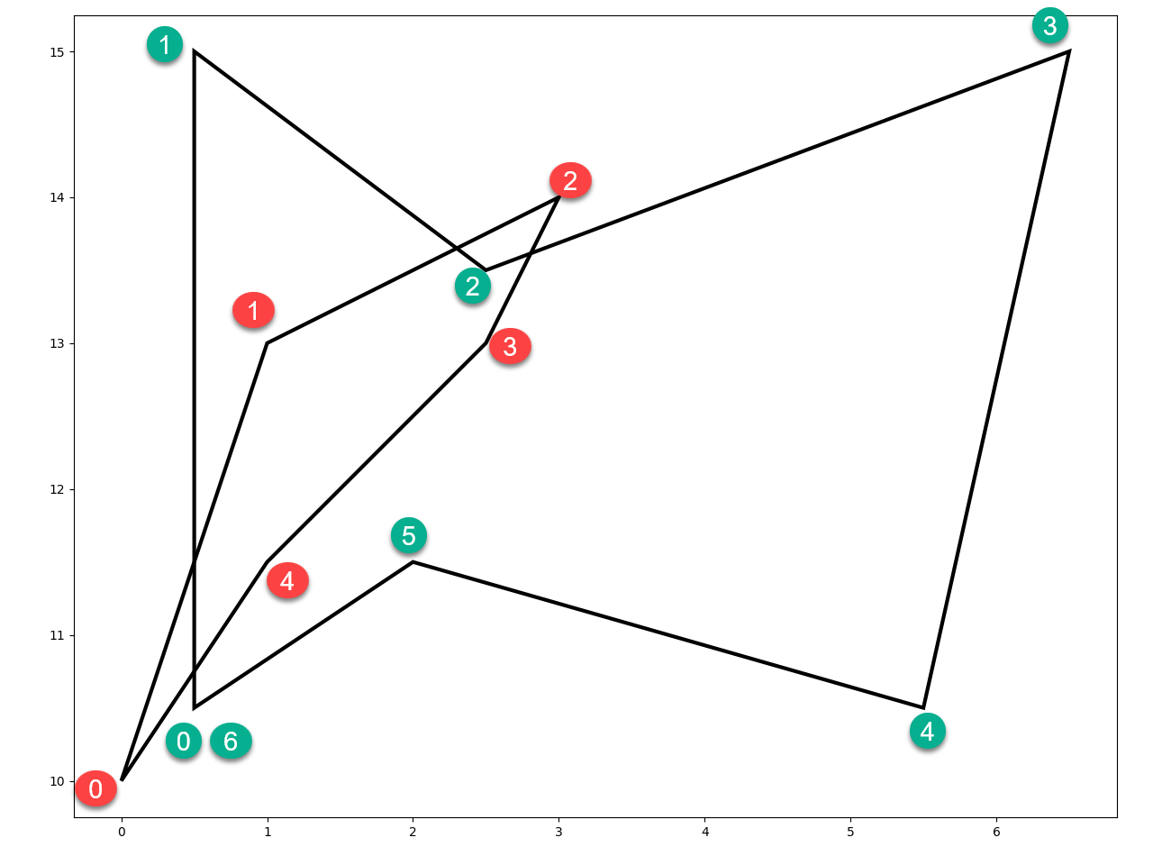
To answer these questions observe the red and green point markers numbered in clockwise order for each of the two polygons.

Our brain can quickly decide which side IF we know the sidedness rule.

If the segments are ordered clockwise, then any point will be inside if it is to the right. If the polygon that we are testing as the home for the points is convex, then an inside point will be to the right of all the line segments.

This is the principle behind the winding number test for point inclusion. It, however, accounts for idiosyncracies that are associated with concave polygons.

Looking at sides

The _side_ code listed below, returns four values.

r : the side array
inside : the points inside (right of) a segment
outside : the points outside (left of) a segment
equal_ : any points that may intersect (equal to) one another by virtue of their equality or potential intersection on the segment.

# check b4 for inclusion in c1
b4                             c1 
array([[  0.00,  10.00],    array([[  0.50,  10.50],
       [  1.00,  13.00],           [  0.50,  15.00],
       [  3.00,  14.00],           [  2.50,  13.50],
       [  2.50,  13.00],           [  6.50,  15.00],
       [  1.00,  11.50],           [  5.50,  10.50],
       [  0.00,  10.00]])          [  2.00,  11.50],
                                   [  0.50,  10.50]])

The coordinates for b4 are used here to just represent points. They actually form a polygon, yet they need not.

The c1 array represents a polygon, as per previous definition.

The _side_ function returns the set of values shown below. r is the cross-product array, which is used to determine parameters.

Two versions of determining points inside (in_ and inside) are calculated. in_ incorporates winding-number calculations for point inclusion in polygons. It is interesting to examine under what circumstances these parameters are similar or different.

r, in_, inside, outside, equal_ = _side_(b4, c1)

r
array([[  2.25, -10.75, -10.25, -24.25,   7.25,   0.25],
       [ -2.25,  -3.25,   0.25, -22.75,  -4.25,  -3.25],
       [-11.25,   1.75,   1.25, -14.75,  -9.75,  -2.75],
       [ -9.00,  -1.00,  -2.00, -16.00,  -5.75,  -1.75],
       [ -2.25,  -6.25,  -5.75, -21.25,   1.00,  -1.00],
       [  2.25, -10.75, -10.25, -24.25,   7.25,   0.25]])

(r < 0)                      r > 0
array([[0, 1, 1, 1, 0, 0],   array([[1, 0, 0, 0, 1, 1],
       [1, 1, 0, 1, 1, 1],          [0, 0, 1, 0, 0, 0],
       [1, 0, 0, 1, 1, 1],          [0, 1, 1, 0, 0, 0],
       [1, 1, 1, 1, 1, 1],          [0, 0, 0, 0, 0, 0],
       [1, 1, 1, 1, 0, 1],          [0, 0, 0, 0, 1, 0],
       [0, 1, 1, 1, 0, 0]])         [1, 0, 0, 0, 1, 1]])

inside                     outside                    equal_
array([[  2.50,  13.00]])  array([[  0.00,  10.00],   array([],
                                  [  1.00,  13.00],         shape=(0, 2),
_in_                              [  3.00,  14.00],          dtype=float64)
array([[  1.00,  13.00],          [  1.00,  11.50],
       [  2.50,  13.00],          [  0.00,  10.00]])
       [  1.00,  11.50]])

# -- calculate in_ using winding number 
_wn_(b4, c1)
array([[  1.00,  13.00],
       [  2.50,  13.00],
       [  1.00,  11.50]])
array([ 0, -1,  0, -1, -1,  0]))
#
lt0 = (r < 0).all(axis=-1)  # array([0, 0, 0, 1, 0, 0])
gt0 = (r > 0).any(-1)       # array([1, 1, 1, 0, 1, 1])
eq0 = (r == 0).any(-1)      # array([0, 0, 0, 0, 0, 0])

side the code

The number of points in each geometry object need not be the same since array-broadcasting is used to facilitate the calculations.

A term like y0[:, None] and other variants change the shape and dimension of the array as follows:

y0  # -- the base array
# y0.ndim  : 1
# y0.shape : (6,)

array([ 10.00,  13.00,  14.00,  13.00,  11.50,  10.00])

# reshape to produce a column array.
y0[:, None]  # ndim = 2, shape = (6, 1)

array([[ 10.00],
       [ 13.00],
       [ 14.00],
       [ 13.00],
       [ 11.50],
       [ 10.00]])

# reshape to change the row array to a 2D array... note the additional [ ] around the coordinates
y0[None, :]  # ndim = 2, shape = (1, 6)

array([[ 10.00,  13.00,  14.00,  13.00,  11.50,  10.00]])

If you start with 2D arrays, then the transitions move them to 3D arrays.

pnts[:, None]
# ndim = 3
# shape = (6, 1, 2)
#
array([[[  0.00,  10.00]],

       [[  1.00,  13.00]],

       [[  3.00,  14.00]],

       [[  2.50,  13.00]],

       [[  1.00,  11.50]],

       [[  0.00,  10.00]]])

pnts[None, :]
# ndim = 3
# shape = (1, 6, 2)
#
array([[[  0.00,  10.00],
        [  1.00,  13.00],
        [  3.00,  14.00],
        [  2.50,  13.00],
        [  1.00,  11.50],
        [  0.00,  10.00]]])

The principles of _side_ are used in subsequent code examples for polygon splitting, clipping and other overlay operations.

def _side_(pnts, poly):
    """Return points inside, outside or equal/crossing a convex poly feature."""
    if pnts.ndim < 2:
        pnts = np.atleast_2d(pnts)
    x0, y0 = pnts.T           # the x and y points
    x2, y2 = poly[:-1].T      # poly segment start points
    x3, y3 = poly[1:].T       # poly segment end points
    r = (x3 - x2) * (y0[:, None] - y2) - (y3 - y2) * (x0[:, None] - x2)
    # -- from _wn_, winding numbers for concave/convex poly
    chk1 = ((y0[:, None] - y2) >= 0.)
    chk2 = (y0[:, None] < y3)
    chk3 = np.sign(r).astype(np.int)
    pos = (chk1 & chk2 & (chk3 > 0)).sum(axis=1, dtype=int)
    neg = (~chk1 & ~chk2 & (chk3 < 0)).sum(axis=1, dtype=int)
    wn_vals = pos - neg
    in_ = pnts[np.nonzero(wn_vals)]
    inside = pnts[(r < 0).all(axis=-1)]  # all True along row, convex polys only
    outside = pnts[(r > 0).any(-1)]      # any True along row
    equal_ = pnts[(r == 0).any(-1)]      # ditto
    return r, in_, inside, outside, equal_